Overview

This is a summary with of a book Exploratory Data Analysis by John W. Tukey, with additional comments from myself. When the book is written in the 70s, computing power (i.e. graph software, or data-related software) was not available for the public, let alone for researchers and analysts. Thus, the majority of the contents were dedicated to pen-and-paper methods, which I am going to omit throughout the whole summary. With that said, I believe the key concepts and ideas for analyzing and visualizing data haven’t change much since then, as visual perceptions of human beings should’ve not undergo dramatic changes. Therefore, it should be useful for this summary to concentrate more on the conceptual basis, rather than the specific techniques for analysis.

Preface

• It is important to understand what you can do before you learn to measure how well you seem to have done it.
• This book is about exploratory data analysis, about looking at data to see what it seems to say. Its concern is with appearance, not with confirmation, to make it more easily handleable by human minds.
• The greatest value of a picture is when it forces us to notice what we never expected to see.

1. Scratching down numbers (stem-and-leaf)

• Exploratory data analysis (EDA) is detective work
  • Needs both tools and understanding
  • Different detailed understandings are needed for each case (Domain knowledge)
• Exploratory vs. Confirmatory
  • Uncovers indications vs. Proves indications to draw out conclusions
  • More flexible vs. More exact
  • We need both; first EDA (search, explore), then CDA (prove, confirm)
• A batch of numbers: a set of similar values
• Stem and leaf method
  • 
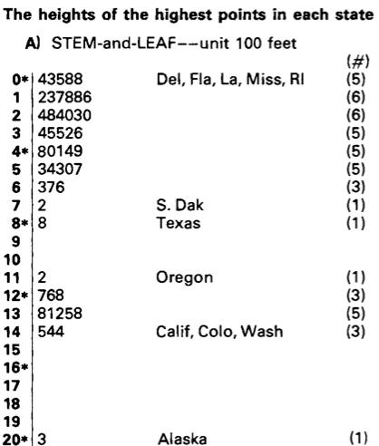
  • Appearances of seperation into groups (clustering)
  • Where the values are centered for each cluster
  • How widely the values are spread for each cluseter
  • Apparent “breaks” (edge values of clusters)
  • Unexpectedly popular or unpopular values
• It is easy to understand numbers, but it is hard to find out what those numbers really imply.

2. Easy summaries — numerical and graphical

• Summarizing the most frequently occuring characteristics of the pattern of a batch
  • Median(Q2), Extremes (min, max), Hinges (quartiles, Q1, Q3)
  • Range: difference between extremes
  • H-spread: difference between hinges
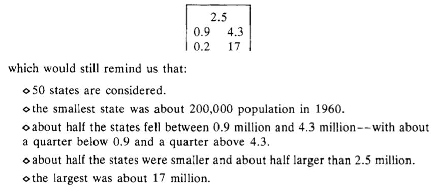
• It would be wrong to expect a standard summary to reveal the unusual.
• There will be no substitute for having the full detail, set out in as easily managable way.
• 5-number summary
  • 
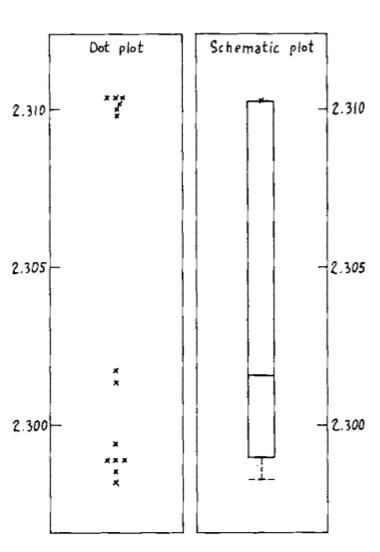
• Dot plot and Box-and-whisker plot
  • 

3. Easy re-expression

• If the way the numbers are collected does not ake them easy to grasp, we should change them, preserving as much information as we can use.
• Re-expressions preserving the ordering: log, sqrt, negative exponentials($-1/x, -1/x^2, -1/x^{1/2}, …$)
• 
• 
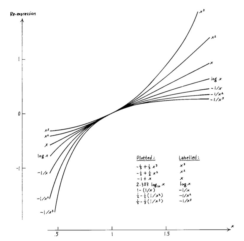
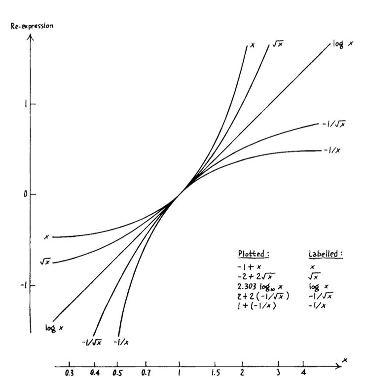
• If one expression is straight, those above it are hollow upward, those below it are hollow downward.
• Can re-express not only the y-axis, but also the x-axis. Any axis can be re-expressed.

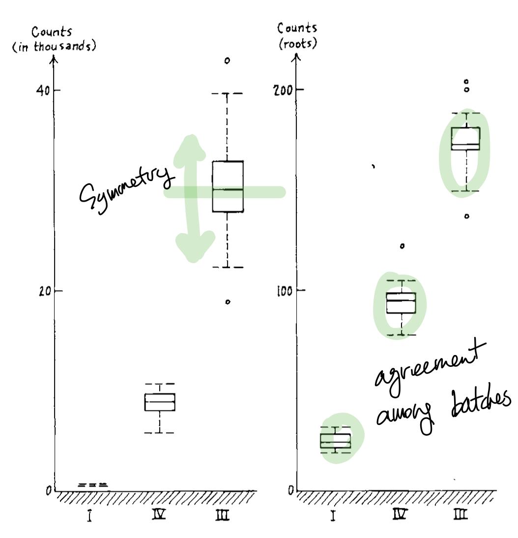
4. Effective comparison, including well-chosen expression

• Choose a good re-expression based on the following
  • Does it show symmetry within each batches well?
  • Does it show agreement among each batches well?
  • 
• Residual = Given value - Summary value (ex. median)
• The meaning of logarithms
  • Reduces multiplications into additions.
  • log residuals are, in fact, ratios

5. Plots of relationship

• Given = Fit + Residual
  • Fit: An incomplete, approximate description. Part of the information. (ex. $y=ax+b$)
  • Residual: Deviation from the current description. Additional information for each point.
  • How it deviates from the description (model) = How it behaves out of the ordinary (generally)
• Using multiple linear models paired with re-expressions
  • 
  • 
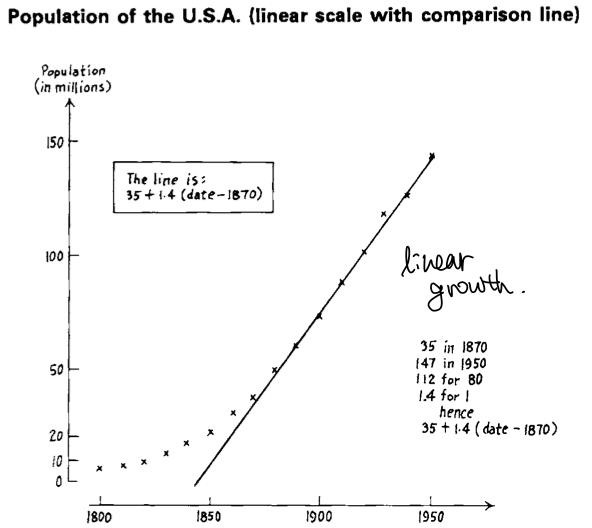
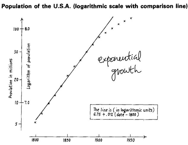
  • The reason behind choosing these models to make a successful approximation, is that we already know these are population data, so we can apply demographic theory, or in other words, domain knowledge for that specific data.
• Indications for re-expressions
  • 

6. Straightening out plots

• Straightening by re-expressing x is not the same as re-expressing y.
• Just because re-expression makes things quite straight, it doesn’t say that it is a new law.

7. Smoothing sequences

• Given data = Smooth + Rough
  • Smooth: Smoothing models such as running medians or moving average. Connected points or smooth curve.
  • Rough: Seperate points.
• Any kind of smoothing methods (or predictive models) has some sort of judgement whatsoever. Eye-smoothing is the maximal amount of judgement, and minimal amount of arithmetic.
• Re-expression does alter the smoothness, but not very much.

8. Parallel and wandering schematic plots

• Median of n shows long-term tendency of length n.
  • We expect to smooth x whenever we smooth y.
  • 
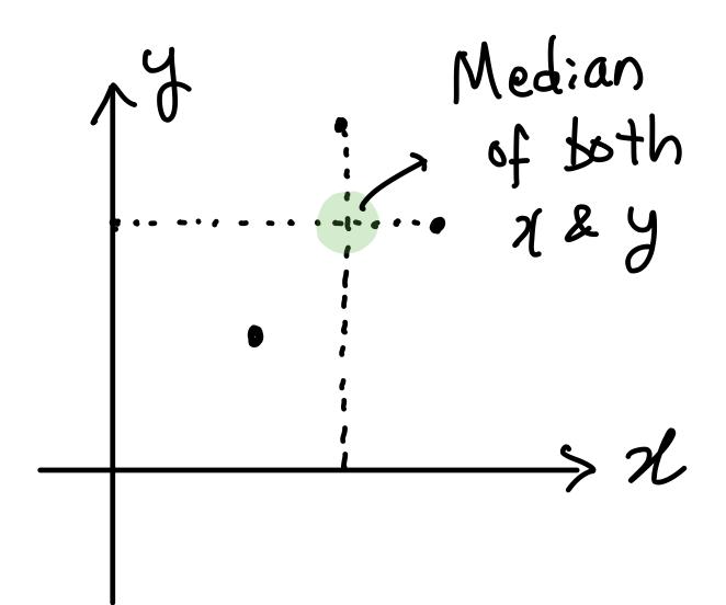
  • Median of both x and y to take the influence of both x and y into account.
• Use h-spread or hinge to model the residual iteslf. (How much it deviate from the smooth model? The roughness of the data.)
• Representative value & Spread = Average (or median) & Quartile = Box & Whisker

9. Delineations of batches of points

• Delineations: Additional traces to model residuals efficiently.
• Failing to show residuals is an essential characteristic of any smooth model.

10. Using two-way analyses

• One kind of response, two kinds of circumstances
  • 
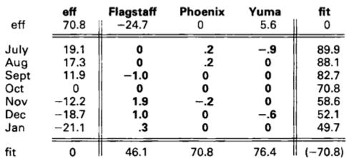
  • data = common + row effect + column effect + residual
  • common (global median) + row effect (row median) + column effect (column median) = median surface
• row + col + 1 fit
  • Modeling with medians
  • $ all + row + col + k \frac {row \times col} {all} $
  • Expression between 1st and 2nd order Taylor expansion
    • 1st (linear combination): $ax + by + c$
    • 2nd: $ax^2 + bx + cy^2 + dy + exy + f$
  • $xy$ term: Covariate term between $x$ and $y$. Simplest and probably most effective nonlinearity.
  • $x^2$, $y^2$ term: Have to remove (or minimize) with re-expression