What is a Manifold?

This is the summary of the lecture, What is a Manifold?, by Dr. Bijan Haney, also known as XylyXylyX. The lecture primarily focuses on constructing a mathematical basis for understanding general relativity, but I was more interested in the deep learning aspect of it. So, do keep in mind that some of the content is missing.

Lecture 1. Point Set Topology and Topological Spaces

Motivation

• Consider two sets: $X = \mathbb{R}^2$ and $Y = (0, 1)$.
  • Even though we are talking about set of points, we are implying its structure. Topology gives structure to a set of points.
• Example structure: Metric $d(p_1, p_2)$ ($\neq$ vector space’s metric).
  • $p_1$, $p_2$ might contain coordinates such as (x, y), but we don’t care about that. We are just defining a function $d$ that is well-defined within $\lbrace(p_1, p_2): p_1 \in S$ and $p_2 \in S \rbrace$ where $S$ is the point set.

Topology?

• Topology $T_X$ for the point set $X$: Also a set!
  • We denote $T_X$ = {Subsets of $X$ (i.e., open set)}
  • Open set of X = Element of the topology for the point set X
  • $(X, T_X)$: Topological space
• Given any sets $u_1, u_2, u_3 \in T_X$,
  1. $u_1 \cup u_2 \in T_X$ (i.e., arbitrary union, possibly infinite)
  2. $u_1 \cap u_2 \in T_X$ (i.e., finite intersections)
  3. Null set $\emptyset \in T_X$ (i.e., smallest set)
  4. $X \in T_X$ (i.e., biggest set)

Example of Topological Spaces

Consider open sets of $\mathbb{R}^2$.

Usual Topology

• Consider the base open ball $ { x: \vert x-p\vert < r } $. For any point p, any radius r, they are all open sets!
• But using only the current defn. Violates (1) and (2) $\to$ We need to include intersections/unions of open balls
• Any shape can be built by correctly union-ing open balls.
  • Example. Rectangle (because we allow infinite union-ing)
  • Example. Intersection of two open ball which can be built by both (1) (obviously…) and (2) (by carefully constructing sets to intersect by unions)
  • Example. Disjoint union (it’s not “connected”, but still an open set)
• Individual point is NOT an open set, because we cannot arrange it without infinite intersection. We only allow finite intersections.

Other Topologies

• Let the defn. of open set = point p. Then, $T_X$ becomes the power set of X $\to$ Discrete Topology
• Let the defn. of open set = {Null, X} $\to$ Trivial Topology
• Open sets of (0, 1)
  • Let the def. of open set: (0, 1-1/N) where N: 2, 3, 4, …
  • We also include the null set to avoid violating (3).
  • For N $\to \infty$, it becomes (0, 1). Hence, it doesn’t violate (4).
  • Their union/intersection will always be the bigger/smaller one, so it doesn’t violate (1) and (2)
  • The size of the base set = size of the open set (i.e., don’t need further intersections/unions to describe the open set. Very rare case, strange topology!)

TL;DR: Definition of topology is arbitrary. If it satisfies the four rules, they are all topologies.

Lecture 2. Elementary Definitions

Defn. Neighborhoods

• For point p in X, we call S the neighborhood of p, when:
  1. S is the subset of X
  2. $p \in S$
  3. For bigger subset $N \supset S$, N is also the neighborhood of p.
  4. For the neighborhoods of p, S and R, $S \cap R$ is also the neighborhood of p.
  5. For the subset $T_p \subset S_p$ where both are neighborhoods of p, and for all point $r \in T_p$, $S_p$ contains the neighborhoods of $r$.

Defn. Closed set

• Closed set is the complement of an open set.
• For any closed set C, $X-C = U$: open set, and $X-U = C$: closed set.

Defn. Limit point

• Thm. Open set that contains p = Open neighborhood of p
  • Remark. For all point in the open set, open set is the open neighborhood for each of the points.
• For a subset $S \subset X$, p is the limit point of S if:
  • For every open neighborhood $u_p$ of $p$,
  • $u_p \cap S - \lbrace p\rbrace \neq \emptyset$.
• Note. S doesn’t need to be the open set.
• Remark. For any boundary point p of open set S (p is not inside S but at the “boundary”), p is the limit point of S. In other words, limit point p do not need to be inside S.
• Remark. If we assume the space $X$ is metric, then the limit point $p$ is a point which has points of $S$ other than itself, arbitrarily close to it.
• Idea. Three edge cases:
  1. “Edge” of $S$: It is a limit point
  2. “Hole” (missing point) “inside” $S$: It is a limit point
  3. “Isolated” point “outside” $S$: It is not a limit point

Defn. Closure

• Given the topological space $(X, T_X)$ and the subset $S \subset X$,
  • $\bar{S}$ (Closure of S) $ = S \cup$ “all of its limit points”
• Idea. It fills up all the edges and holes of $S$. “Isolated” is already inside $S$.

Defn. Interior

• Point $p \in S^0$ (the interior of the set S) if:
  • I can find a subset $u_p \subset S$ that is the open set containing p.
• Note. For the usual topology, “edge” is not inside the interior, even in the case when S is the closed set.
• Remark. $S^0$ is always open.
• Remark. $S^0$ is the union of all the open sets inside S.
• Remark. S is open if and only if $S = S^0$.
• Remark. $S^0 = {\overline{S^c}}^c$. In other words, $S^0$ is the complement of the closure of the complement of S.
  • Complement of S = Outside S (Includes “holes”)
  • Closure of the complement of S (Includes “edges”)
  • Complement of the closure of the complement of S (Excludes “edges” and “holes.”)
• Idea. All three edge cases $\notin S^0$.

Defn. Exterior

• Complement of its closure $\overline{S}^c$
• Idea. Three edge cases $\notin \overline{S}^c$
  1. “Edge” and “Hole” is not the exterior because it’s “too close” to the set $S$.
  2. “Isolated” is not the exterior because it’s not “outside” $S$.

Defn. Boundary

• Neither the exterior nor the interior.
• Remark. It includes all the three edge cases.

Defn. Dense

• For a subset $S \subset X$, S is dense in X when:
  • For all point $p \in X$, $p \in S$ or p is the limit point of S.
  • In other words, $p \in \bar{S}$.
• Example. Consider the set of points with rational coordinates $S = \lbrace(q_1, q_2) \vert q_1 \in \mathbb{Q} \text{ and } q_2 \in \mathbb{Q}\rbrace$.
  • S is dense in the usual topology of $\mathbb{R}^2$, because we can find an infinitely close rational number (neighborhood) for any irrational number.
  • However, S is not dense in the discrete topology.

Lecture 3. Alternative Topologies and Separation

Alternative Topologies for Intervals

• We introduce various example topologies to understand different concepts more clearly.
• Recall. Topologies for open interval (0, 1)
  • Usual topology $T_E$: Open interval (Euclidean topology)
  • “Nested interval” topology $T_{NI}$: (0, 1-1/N) where N: 2, 3, …

Closed Interval Topology $T_{CI}$

• Consider the topology $T_{CI}$ for the closed interval $[-1, 1]$.
  • Let’s set the bases as half-open intervals $[-1, a)$ and $(b, 1]$ where $a>0, b<0$.
    • Let’s denote the former “lower base” and the latter “upper base.”
  • Union/Intersection within the lower/upper base is just the bigger/smaller member (same with the “Nested interval” topology).
  • Union of the any member of the lower & upper base is always the entire set.
  • Intersection of the upper & lower element: open interval (b, a) which always includes “0.” Hence, it’s not a “general” open interval.

Cofinite Topology $T_{CF}$

• For the open interval $X$ (0, 1) with the usual topology $T_X$:
  • Choose the finite number of points. Its complement can be constructed by the following:
    • Example. Points = {0.2, 0.4}. Then, the complement of the points = (0, 0.2) $\cup$ (0.2, 0.4) $\cup$ (0.4, 1.0) $\in T_X$.
  • We can exclude the finite number of points.
    • Example. ${0.2, 0.4}^C \cap {0.3, 0.4}^C = {0.2, 0.3, 0.4}^C$

Separability

$T_0$ Separability (Kolmogorov)

• To satisfy the $T_0$ Separability:
  • For any two points $p_1, p_2 \in X$, there has to exist an open set $S \in T_X$ such that $p_1 \in S$ but $p_2 \notin S$.
  • In other words, there has to exist the open set that distinguishes two points.
• Remark. $T_E$ satisfies it.
• Remark. $T_{NI}$ does not satisfy it.
  • Consider $p_1=0.1, p_2=0.2$.
  • The bases are (0, 0.5), (0, 0.67), (0, 0.75)…
  • Hence, $p_1$ and $p_2$ is always within the base (0, 0.5). $\to$ Violation!
• Remark. $T_{CI}$ satisfies it.
  • For the case where $p_1>0, p_2<0$, $T_{CI}$ can be separated by using either lower or upper base.
    • This is somewhat stronger than $T_0$, because we can find separate open set for both points.
  • For the asymmetric case where $p_1 * p_2 > 0$, it can be separated by using lower/upper base only.

$T_1$ Separability (Frechet)

• To satisfy the $T_1$ Separability:
  • For any two points $p_1, p_2 \in X$, there has to exist open sets $\mathbf{S_1, S_2} \in T_X$ such that $p_1 \in S_1, p_2 \notin S_1$ and $\mathbf{p_1 \notin S_2, p_2 \in S_2}$.
  • In other words, each has to have a neighborhood not containing the other point.
• Remark. $T_{CF}$ satisfies it.

$T_2$ Separability (Hausdorff)

• To satisfy the $T_2$ Separability:
  • For any two points $p_1, p_2 \in X$, there has to exist disjoint open sets $S_1, S_2 \in T_X$ and $\mathbf{S_1 \cap S_2 = \emptyset}$,
  • such that $p_1 \in S_1, p_2 \notin S_1$ and $p_1 \notin S_2, p_2 \in S_2$.
• Remark. $T_{CF}$ does not satisfy it, but $T_E$ satisfy it.
• The most common one! Also, if you want, you can get more stronger separability than this.

Interesting properties

• Consider the usual topological space $(\mathbb{R}^2, T_E)$ and the real line $L \subset \mathbb{R}^2$ on the space.
  • Subset L induces a new usual topological space $(L, T_L)$ as all the open sets in $T_L \subset T_E$ (i.e., the neighbors of the boundary L) acts as an open interval.
• Consider the topological space $(U, T_U), (S, T_S)$.
  • The cartesian product $U \times S$ has the topology $T_U \times T_S$.

Lecture 4. Countability and Continuity

Countability

Motivation

• Consider the topological space $(X, T)$ and a point $p \in X$ inside the open set $S \in T$.
• Let’s define a more smaller open set $S_1 \subset S$ that is the neighbor of $p$.
• Let’s keep defining the smaller open set such that $S_{n+1} \subset S_n$.
• The nested collection could terminate (ex. Discrete Topology), but for the open ball topology, there will be an infinite number of open sets.

Defn. First-Countability

• The topological space $(X, T)$ is first-countable when:
  • For every point $p \in X$, there exist a countable open nested neighborhoods.
• Remark. If we use rational coordinates on the usual topological space, we can build a countable nested collection such as a ball with radius 1/N, i.e., usual topological space is first-countable.

Defn. Second-Countability

• The topological space $(X, T)$ is second-countable when the topology has a countable base, i.e.,
  • For every open set $S \in T$ can be written as $S = \cup_i b_i$ of the bases $b_i$.
• Remark. If we use rational coordinates on the usual topological space, we can define a “rational” neigborhood for every point $p \in X$, i.e., usual topological space is second-countable.

Remarks

• If the space is second countable, it is always first-countable. However, the converse is not true.
• Manifolds that “behave well” is second-countable.
• Nested interval topology $T_{NI}$ and closed interval topology $T_{CI}$ are second-countable.
• Cofinite topology $T_{CF}$ is not first-countable. (Approach: Start with a basis, check whether one can build a smaller basis based on the initial one.)

Example. Lower-limit Topology $T_{LL}$

• Consider a lower-limit topology with the basis set $[b, a) \in T_{LL}$.
  • Note that $(l, m) \in T_{LL}$ by the following construction:
  • Consider a sequence $b_n \to l^+$. Then, the infinite union $\cup_n^\infty [b_i, m) = (l, m)$.
• Remark. Euclidean topology $T_E \subset T_{LL}$. In other words, $T_LL$ is finer to $T_E$ and $T_E$ is coarser to $T_{LL}$.
• Remark. It is clearly first-countable. However, it is not second-countable.
  • Assume that there exists a countable basis $[b_n, a_m)$ where $n, m \in \mathbb{I}$.
  • One can only construct a basis that is customized to a specific $(l, m)$. If we change $l$, we have to redefine $b_n$, which violates the assumption of a fixed countable basis.
• “There is always this weird counterexamples.”

TL; DR: This is why we want the manifolds to be Hausdorff & Second-countable, because, if not, weird things happen.

Continuity

Motivation

• Consider a function $f: X \to Y$ where $X, Y$ is endowed to each topologies $T_X, T_Y$.
• We want to define continuity of the function $f$.
• Recall. epsilon-delta definition of a limit assumes lots of information such as the existence of a distance function. We aim to define continuity without these.

Defn. Continuity

• Consider the inverse mapping $f^{-1}$ and the arbitrary open set $S_Y \in T_Y$.
• A function $f$ is continuous if the pre-image $f^{-1}(S_Y)$ is an open set in $T_X$.
• Remark. Relation with the epsilon-delta
  • [epsilon-side] For any $S_Y \in T_Y$,
  • [delta-side] we need to find the tight-enough open neighborhood $S_X \in T_X$ such that $f(S_X) \subset S_Y$.

Examples

• Consider the function $f(x)=x$ and the topologies $T_E, T_{NI}, T_{CI}, T_{CF}, T_{LL}$.
  • Recall. Euclidian, Nested Intervals, Closed Intervals, Cofinite, Lower Limit
  • Each bases: (a, b), (0, 1-1/N), [-1, a) and (b, 1], Point exclusion, [b, a)
• $T_E \to T_{NI}$: Inverse of the nested interval (0, 1-1/N) directly maps to (a, b), i.e., for all the open set of $S_Y \in T_Y$, $f^{-1}(S_Y) \in T_X$. Hence, $f$ is cont.
• $T_E \to T_{CI}$: Open intervals are okay, But, it fails on the form of [0, a) or (b, 1] due to the point 0, 1. Hence, $f$ is not cont.
• $T_E \to T_{CF}$: N open intervals’ union ($\in T_{CF}$) maps fine to $T_E$. Hence, $f$ is cont.
• $T_E \to T_{LL}$: Half-closed interval [a, b) is not a closed set in $T_E$. Hence, $f$ is not cont.
• $T_{NI}, T_{CI}, T_{CF} \to T_E$: Consider (0.1, 0.2). It fails on everything.
• $T_{LL} \to T_E$: $f$ is cont. Recall that $T_{LL}$ is finer to $T_E$.
• Everything else to $T_{Distinct}$: $f$ has to be cont. because $T_{Distinct}$ is the finest topology.
• $T_{Distinct} \to T_{LL}$: Consider [0.1, 0.2]. Due to the upper limit, it fails. Hence, $f$ is not cont.

Lecture 5. Compactness, Connectedness, and Topological Properties

Defn. Homeomorphism

• Defn. $f$ is homeomorphic when:
  • $f$ and $f^{-1}$ is both the cont. function, 1-to-1, and onto.
• Recall.
  • 1-to-1 (injection): if $f(a) = f(b)$, $a=b$. In other words, if $a \neq b$, $f(a) \neq f(b)$.
  • Onto (surjection): Image is equal to its codomain.
• Remark. This is important because various topological properties are preserved for homeomorphisms, such as separability, connectedness, or compactness.
• Remark. There is no sense of shape, metric, and geometry here. It is very abstract.

Defn. Compactness

• Defn. Open cover of a set X = A collection of open sets (subcovers) whose union covers X, i.e., $X \subset \cup_i s_i$.
• Case 1. Consider the case where the number of subset needs to be infinite to cover the open set X.
  • For example, next subcover only half of the remaining X that is not covered by the sum of previous subcovers.
  • Excluding the boundary, the subsets will eventually cover all the elements in open set X, approaching the boundary as close as possible.
• Case 2. Compare it with the case where there are infinite number of subcovers, but only need finite subset of them to actually cover X.
• Defn. If I find any cover that needs infinite number of subcovers to cover X (Case 1), we call X not compact.
• Case 3. Same with Case 1, but with the closed set X.
  • Because of the boundary, the subcovers will get infinitely close to the boundary, but never include the boundary.
  • To include the boundary, we need to come up with a subcover that includes the boundary. It will touch the progressing subcovers, hence making the total number of subcovers finite.
  • Remark. One cannot found that is infinite. This case is compact.

Defn. Connectedness

• For the topological space $(X, T_X)$, if there exists open sets $G, H \in T_X$ such that $G \cap H = \emptyset$ and $G \cup H = X$, we call that X is not connected.
  • Remark. If there are two or more disconnected subset, we call X not connected.
• Remark. Homeomorphism $f$ preserves connectedness.
  • For the topological space $(Y, T_Y)$ and function $f: X \to Y$, $f(G), f(H) \in T_Y$, $f(G) \cap f(H) = \emptyset$, and $f(G) \cup f(H) = Y$.

Defn. Path-connectedness

• Defn. Given the arbitrary point $x, y \in X$, if I can draw a line between $x, y$, we call $x, y$ path-connected.
  • Draw a line means that I can define a continuous function $f: [0, 1] \to X$ where $f(0) = x, f(1) = y$.
• Defn. If I can path-connect arbitrary two points of X, we call X path-connected.
• Remark. If X is path-connected, X is connected. Its converse is not true.
• Remark. If one path can be “continuously deformed” into the other, such a deformation is called a homotopy.
  • On the sphere, any path can be deformed into another path (Simply connected).
  • However, on the donut, if it circles around the hole, it cannot be deformed into the straight path.

Lecture 6. Topological Manifolds

Paracompactness

• Paracompact if every open cover has an open refinement that is locally finite.
• A refinement of a cover C is a new cover D such that every set in D is contained in some set in C.
• Locally finite if each point in the space has a neighbourhood that intersects only finitely many of the sets in the collection.
• Remark. Compactness is a property that seeks to generalize the notion of a closed and bounded subset of Euclidean space by making precise the idea of a space having no “punctures” or “missing endpoints”, i.e. that the space not exclude any limiting values of points.
• Remark. Paracompactness is more of a local property while Compactness is a global property.

Requirements for the Topological Manifold

• We consider the topological space $(X, T_X)$ (Set with its topology)
• with the topological properties:
  • Hausdorff (two points separable with two disjoint open set)
  • Second-countable (has a countable basis)
  • Paracompact (locally closed and bounded)
• which makes the space metrizable.
  • Metrizable = We can invent a metric $d$ that measure the space
  • $d: X \times X \to \mathbb{R}^{+}$ (Sometimes it’s $\mathbb{R}$ such as the Riemannian metric)
  • Hausdorff (to distinguish points in a very aggressive way), Second-countable & Compact (to control the space to make it useful)
• If it’s locally Euclidean, we call the space Topological Manifold.

Motivation for the Locally Euclidean

• $\mathbb{R}^N$ is simply a tuple of N real numbers. So, let’s endow it with the usual topology (i.e., open ball topology), i.e., consider the topological space $(\mathbb{R}^N, T_{\mathbb{R}^N})$, which is quite rich!
• We need to build a homeomorphism from the topological manifold to $\mathbb{R}^N$, i.e., $f: X \to \mathbb{R}^N$, to enjoy its richness.
• Let’s enjoy the simplicity of $\mathbb{R}^N$, yet avoid requiring the extreme requirement of homeomorphism across the whole space by incorporating the idea Locally Euclidean!

Exploiting the locality

• Let’s consider a space $(X, T_X)$ and its open set $U_p$, which is the neighborhood of the point $p$.
• Note that $(U_p, T_X \vert_{U_p})$ is also a topological space: all the elements’ unions and intersections are inside $U_p$, and the total union is equal to $U_p$. We can call that it inherited the topology from the original space.
• Now, consider the open set of $\mathbb{R}^N$, $S, T_{\mathbb{R}^N} \vert_S$ and the homeomorphism $f: U_p \to S$, which is much easier to construct!
• Let’s extend this further. Consider any point $p \in X$ and its corresponding point $f(p) \in \mathbb{R}^N$. It’ll be awesome if we get to design $f$ for every open neighborhood of $p$ and $f(p)$, i.e., for every subcover of the open cover of $X$.
• If we manage to do so, we get to obtain the coordinates, i.e., $X$ is locally Euclidean.
  • Be careful that each subcover maps to a different copy of $\mathbb{R}^N$, so comparing the coordinates across different subcovers won’t make any sense.

Classic example: Earth map

• Consider the surface of the sphere $(X, T_{\mathbb{R}^3}\vert_X)$ which inherits from the 3-dimensional space.
  • We can easily construct $X$ by starting from the open ball $S$. The closure $\bar{S}$ will include the surface, hence let’s subtract the interior: $X=\bar{S} - S^0$.
• Sphere is compact but the plane is not.
  • Hence, we can automatically determine that there will be no homeomorphism from $X \to \mathbb{R}^2$ (because it’ll preserve the topological properties).
  • However, if we remove a single point from $X$, it becomes non-compact! (Consider the continuously halving subcovers example towards the south pole)
• Consider any open neighborhood of the point $p$ on the sphere and its corresponding circle (open neighborhood of $f(p)$) on the plane $\mathbb{R}^2$.
  • Even though the whole sphere is not mappable to $\mathbb{R}^2$, each region is, i.e., locally homeomorphic.
• Let’s directly design the mapping:
  • Exclude the south pole $Q$. Given the north pole $P$, let the neighborhood $u_P = X-Q$.
  • Let the plane pass through the sphere’s center, perpendicular to $\overline{PQ}$. Then, for any point $p$ on $u_P$, I can draw a line $\overline{pQ}$.
  • The intersection of the line and the plane becomes the mapping $\gamma_P$.
  • You can’t map $Q$, but everything else is successfully mapped. It is also homeomorphism, i.e., easily determine its reverse.
  • If we do the same thing by excluding $P$ and including $Q$, we can yield $\gamma_Q$.
  • We can yield the Atlas $\mathcal{A} = \lbrace (u_P, \gamma_P), (u_Q, \gamma_Q) \rbrace$, which is a set of Charts, i.e., tuples of the chart region $u$ and the homeomorphic map $\gamma$.

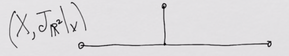
Classic counterexample

• T-shaped line inherited from $\mathbb{R}^2$
  • 
• If we wanted to map this to $\mathbb{R}^1$, the center point’s neighborhood becomes the problem. There is now way to design a homeomorphism without violation on continuity (the center point has to be inside two line segments, which is not possible).
• It also fails for $\mathbb{R}^2$ due to the simple line segment. In $\mathbb{R}^2$, line segment is not an open set.
• The space is not elligible for the topological manifold!

Lecture 7. Differentiable Manifolds

• Recall. Topological manifold space $(X, T_X, \mathcal{A})$ where the atlas $\mathcal{A} = \lbrace (u_i, \gamma_i) \rbrace$. Homeomorphic mapping $\gamma$ maps to the Euclidean space $\mathbb{R}^d$ with dimension $d$, so that the point $p \in X$ is mapped to the coordinates $\gamma_i(p) = (\alpha_i^1, \cdots, \alpha_i^d)$.
• Remark. $X$: real world, $\mathbb{R}^d$: model. We do all of our work on $\mathbb{R}^d$.

Transition function

• Let $\mathcal{A} = \lbrace (u_1, \gamma_1), (u_2, \gamma_2), \cdots \rbrace$, $u_{12} = u_1 \cap u_2$.
  • Remark. Intersections might be quite severe. Recall the Earth map example. Its intersection = everything except the north and the south pole.
  • Remark. You must have overlaps because neighborhoods are open sets, and their boundaries must also be included.
• Point $p \in u_{12}$ is mapped to both $\gamma_1(p) \in u_1, \gamma_2(p) \in u_2$ by each homeomorphisms.
  • Remark. Connectedness is preserved, i.e., no holes.
• Consider a map: $f: \gamma_1(u_{12}) \to \gamma_2(u_{12})$, or in other words, $\mathbb{R}^d \to \mathbb{R}^d$. $f = \gamma_2 \circ \gamma_1^{-1}$. We call $f$ a transition function which translates the coordinates from $u_1$’s corresponding space to that of $u_2$’s.
  • Remark. $f^{-1} = \gamma_1 \circ \gamma_2^{-1}$.

Differentiable Manifold

• Remark. It is guaranteed that $f \in C^0$ ($f$ is continuous).
• Defn. If $f \in C^\infty$ (i.e., $f$ is a smooth function, $f$ is infinitely differentiable), we call the space differentiable manifold $(X, T_X, \mathcal{A})$.
  • Remark. All differentiable manifolds are topological manifolds, but the converse is not true.
  • Remark. We can now enjoy various tools such as multivariate calculus.

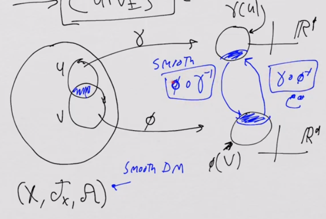
Defn. Compatibility of Charts

• Charts $(u, \gamma)$ and $(v, \phi)$ is compatible when:
  1. $u \cap v = \empty$
  2. $u \cap v \neq \empty$ and both $\phi \circ \gamma^{-1}, \gamma \circ \phi^{-1}$ are smooth
• Remark. If $X$ is a differentiable manifold, every intersecting pair of charts has a smooth transition function, i.e., compatible.
• Consider two different atlases $\mathcal{A}, \mathcal{B}$ that are both compatible. $\mathcal{C} = \mathcal{A} \cup \mathcal{B}$.
  • Obvious result: $\mathcal{C}$ is a valid atlas.
  • Advanced result: $\mathcal{C}$ is a differentiable manifold when $d \le 3$. However, it cannot be guaranteed when $d \ge 5$. There are infinite number of differentiable structures on $d=4$, but finite on $d>4$.
  • Maximal atlas: Union of all atlases where it is compatible. Does not grow bigger and compatible for any other atlas.
  • For every maximal atlas, there is a differentiable structure.

    Summary

    

Lecture 8. Curves, Coordinate Functions, and Diffeomorphisms

Defn. Curve

• Consider a differentiable manifold $(X, T_X, \mathcal{A})$ and any point $\lambda \in \mathbb{R}$ on the real line.
• Let an arbitrary function $f: \mathbb{R} \to X$. We call $f$ the curve.
• Remark. Its range will pass through one or more chart regions.
• Example. Consider two overlapping charts $(u, \gamma), (v, \phi)$. Then, $\gamma \circ f, \phi \circ f: \mathbb{R} \to \mathbb{R}^d $.

Defn. Coordinate function

• Consider a differentiable manifold $(X, T_X, \mathcal{A})$ and a chart $(u, \gamma) \in \mathcal{A}$.
• For any $p \in X$, $\gamma(p) \in \mathbb{R}^d$. We call each function per coordinate $\gamma(p) = (\alpha^1(p), \alpha^2(p), \cdots \alpha^d(p))$ coordinate functions where $\alpha^i: X \to \mathbb{R}$.

Defn. Diffeomorphism

• Consider two differentiable manifold $(X, T_X, \mathcal{A}), (Y, T_Y, \mathcal{B})$ and the function $f: X \to Y$.
• For two charts $(u, \gamma) \in \mathcal{A}, (v, \phi) \in \mathcal{B}$, we can define $\phi \circ f \circ \gamma^{-1}: \mathbb{R}^{d_X} \to \mathbb{R}^{d_Y}$.
• If $f$ exists where it is:
  1. 1-to-1
  2. Onto
  3. Both $f, f^{-1}$ are differentiable
• Or in other words, homeomorphic and differentiable,
• we call $f$: diffeomorphism and $\mathcal{A}, \mathcal{B}$: diffeomorphic spaces.
• Remark. Diffeomorphism = Homeomorphism for differentiable manifolds

Lecture 9. Tangent Space

Settings

• 
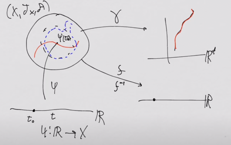
• Consider two differentiable manifolds $(X, T_X, \mathcal{A}), (\mathbb{R}, T_\mathbb{R}, \mathcal{B})$, any chart $(u, \gamma) \in \mathcal{A}$, and a function $f: X \to \mathbb{R}$.
  • Recall. $\gamma: X \to \mathbb{R}^d, f \circ \gamma^{-1}: \mathbb{R}^d \to X \to \mathbb{R}$.
  • Differentiability check: Checking whether $f \in C^\infty$ or not.
  • Note. Let $\mathcal{B} = \lbrace (v_1, \phi_1) \rbrace$. Then, $v_1 = \mathbb{R}$ and $\phi_1 = I_\mathbb{R}$, i.e., identity mapping.
• Consider a curve $\psi: \mathbb{R} \to X$. (Let’s denote $\mathbb{R}$ as $\mathbb{R}_t$ from now on to avoid confusion.)
  • Idea. This is the time dimension in physics.
  • Remark. $\gamma \circ \psi: \mathbb{R}_t \to X \to \mathbb{R}^d, f \circ \psi: \mathbb{R}_t \to X \to \mathbb{R}$.

Velocity

• 
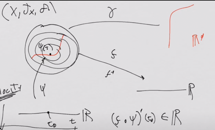
  • We drew contours where $f$ values are the same.
• Consider the amount of change on $f$ with respect to $t$, i.e., $d(f \circ \psi)/dt$ or $(f \circ \psi)’ (t)$.
  • It is dependent on the curve $\psi$. For example, with the different curve, it’ll be totally different.
  • Note. More sloppy notation $df/dt$ is often used in other literature.
• Consider a mapping $v_{\psi, t_0}: C^\infty(X) \to \mathbb{R}$ with the parameters $\psi$ and $t_0 \in \mathbb{R}_t$.
• Then, $v_{\psi, t_0} (f) = (f \circ \psi)’(t_0)$.
• This is the notion of velocity in physics. More formally, it’s a velocity of a function $f$ when passed through by $\psi$ on a single point $t_0$.

Choosing one curve

• 
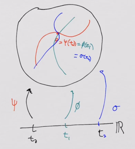
• There will be an infinite varieties of derivatives based on the curve:
  • $v_{\psi, t_0}(f) = (f \circ \psi)’(t_0), v_{\phi, t_1}(f) = (f \circ \phi)’(t_1), v_{\sigma, t_2}(f) = (f \circ \sigma)’(t_2)$.
  • Let a point $p \in X$ where $p = \psi(t_0) = \phi (t_1) = \sigma (t_2)$.
• Hence, let’s define a set of all possible mappings $\lbrace v_{\gamma, t} \vert \gamma: \mathbb{R} \to X \rbrace$, and show that it is a vector space by proving:
  1. (Addition) There exists a mapping $\sigma$ where $v_{\psi, t_0} (f) + v_{\phi, t_1}(f) = v_{\sigma, t_2}(f)$.
  2. (Scalar multiplication) There exists a mapping $\sigma$ where $\alpha \cdot v_{\psi, t_0} (f) = v_{\sigma, t_2}(f)$ for any $\alpha \in \mathbb{R}$.

Proof of 1. Addition

• Claim. $\sigma(t) = \gamma^{-1} \lbrack (\gamma \circ \psi)(t_0 + t) + (\gamma \circ \phi) (t_1 + t) - (\gamma \circ \psi)(t_0) \rbrack$.
  • Note. It works even if we swap $\phi$ with $\psi$.
• Observation. $\sigma(0) = \gamma^{-1}\lbrack \gamma(p) + \gamma(p) - \gamma(p) \rbrack = p$, hence $t_2 = 0$.
• Velocity $v_{\sigma, t}(f) = (f \circ \sigma)’(0) = ((f \circ \gamma^{-1})\circ (\gamma \circ \sigma))’(0)$.
  • Note. We’re derivating with respect to $t$.
  • Note. $\gamma \circ \sigma: \mathbb{R} \to \mathbb{R}^d, f \sigma \gamma^{-1}: \mathbb{R}^d \to \mathbb{R}$.
• (cont.) $v_{\sigma, t}(f) =\sum_j \partial_j (f \circ \gamma^{-1}) (\gamma \circ \sigma(0)) \cdot (\gamma \circ \sigma)_j’(0)$
  • $(\gamma \circ \sigma)_j’(0) = (\gamma \circ \psi)’_j(t_0 + 0) + (\gamma \circ \phi)’_j (t_1 + 0) - \sout{(\gamma \circ \psi)’_j(t_0)}$
  • $\because$ Last term is not dependent on $t$.
• (cont.) $v_{\sigma, t}(f)= \sum_j \partial_j (f \circ \gamma^{-1}) (\gamma (p)) \cdot (\gamma \circ \sigma)j’(0) = \sum_j \partial_j (f \circ \gamma^{-1}) (\gamma (p)) \cdot \lbrack (\gamma \circ \psi)_j’(t_0) + (\gamma \circ \phi)_j’(t_1) \rbrack = (f \circ \psi)’(t_0) + (f \circ \phi)’(t_1) = v{\psi, t_0} (f) + v_{\phi, t_1}(f).$ QED.
  • Remark. $f$ becomes irrelevant, hence it works for an arbitrary chart. Hence, $v_{\sigma, t_2} = v_{\psi, t_0} + v_{\phi, t_1}$.
  • Note. As $p = \psi(t_0) = \phi (t_1) = \sigma (t_2)$, we also write the above as $v_{\sigma, p} = v_{\psi, p} + v_{\phi, p}$.